Video Feedback Simulator
In an effort to learn some Javascript and WebGL, a friend and I put together a video feedback simulator based on lazy afternoons of holding a webcam up to a TV.
If you aren’t concerned about unleashing potentially bright, flashing, animated chaos, you can play with it here.
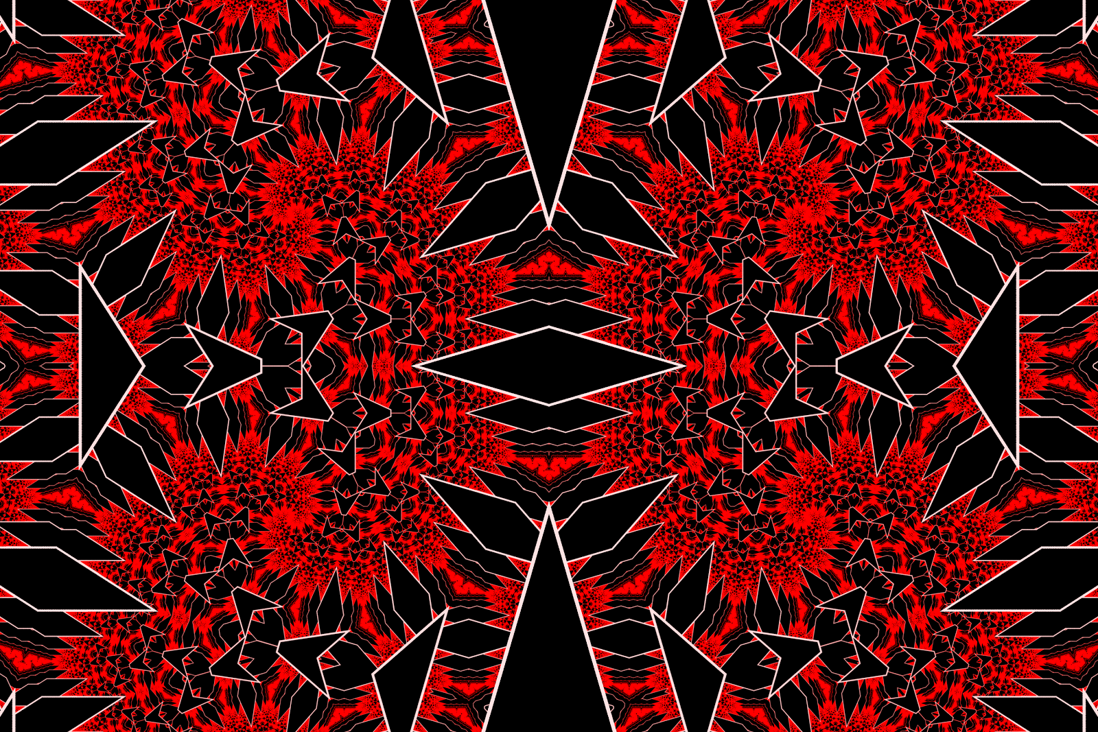
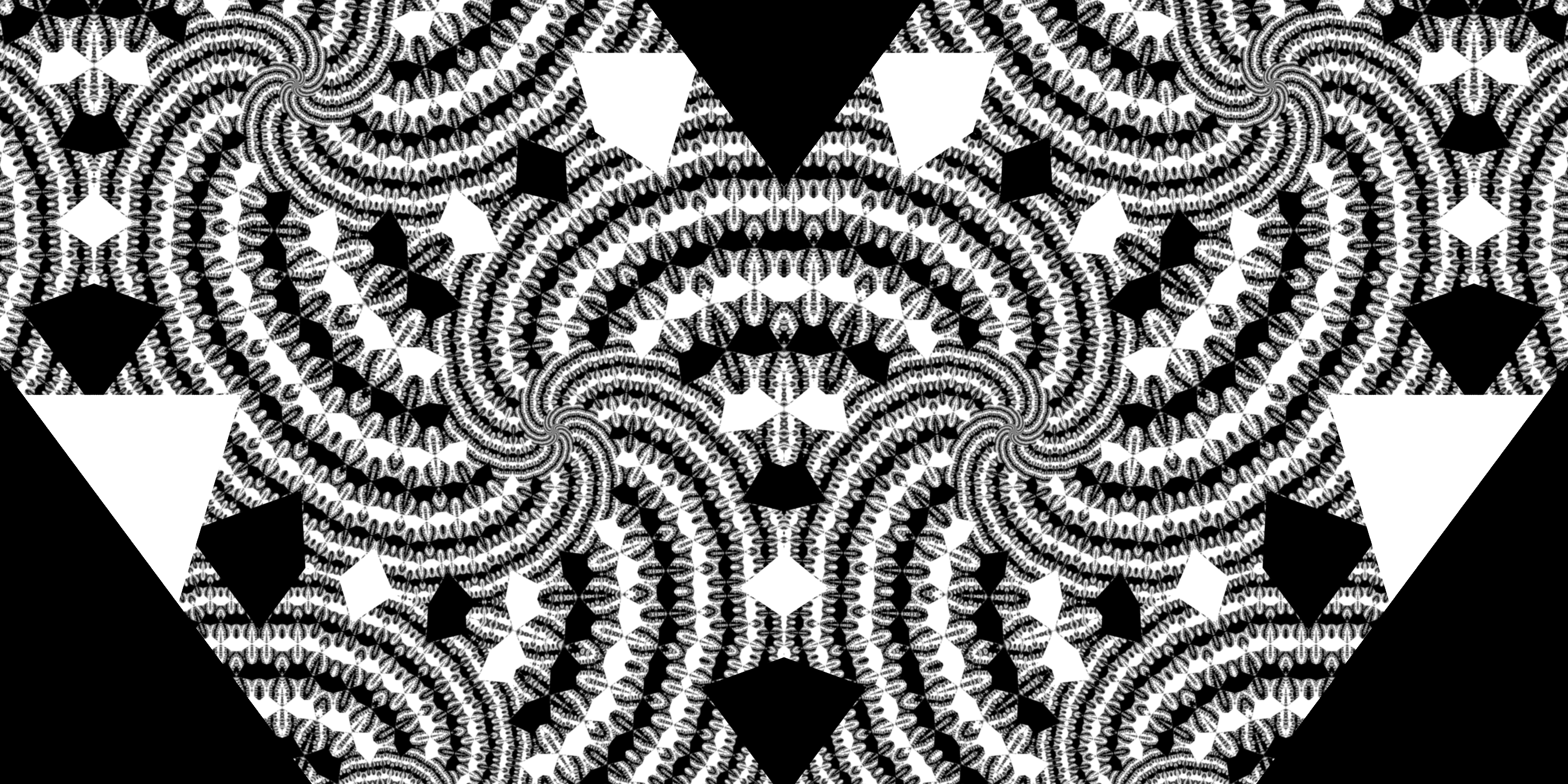
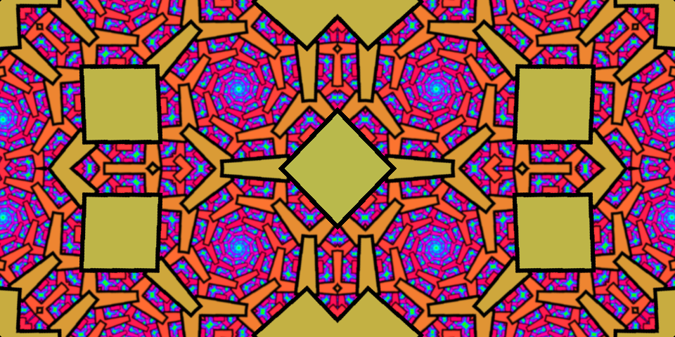
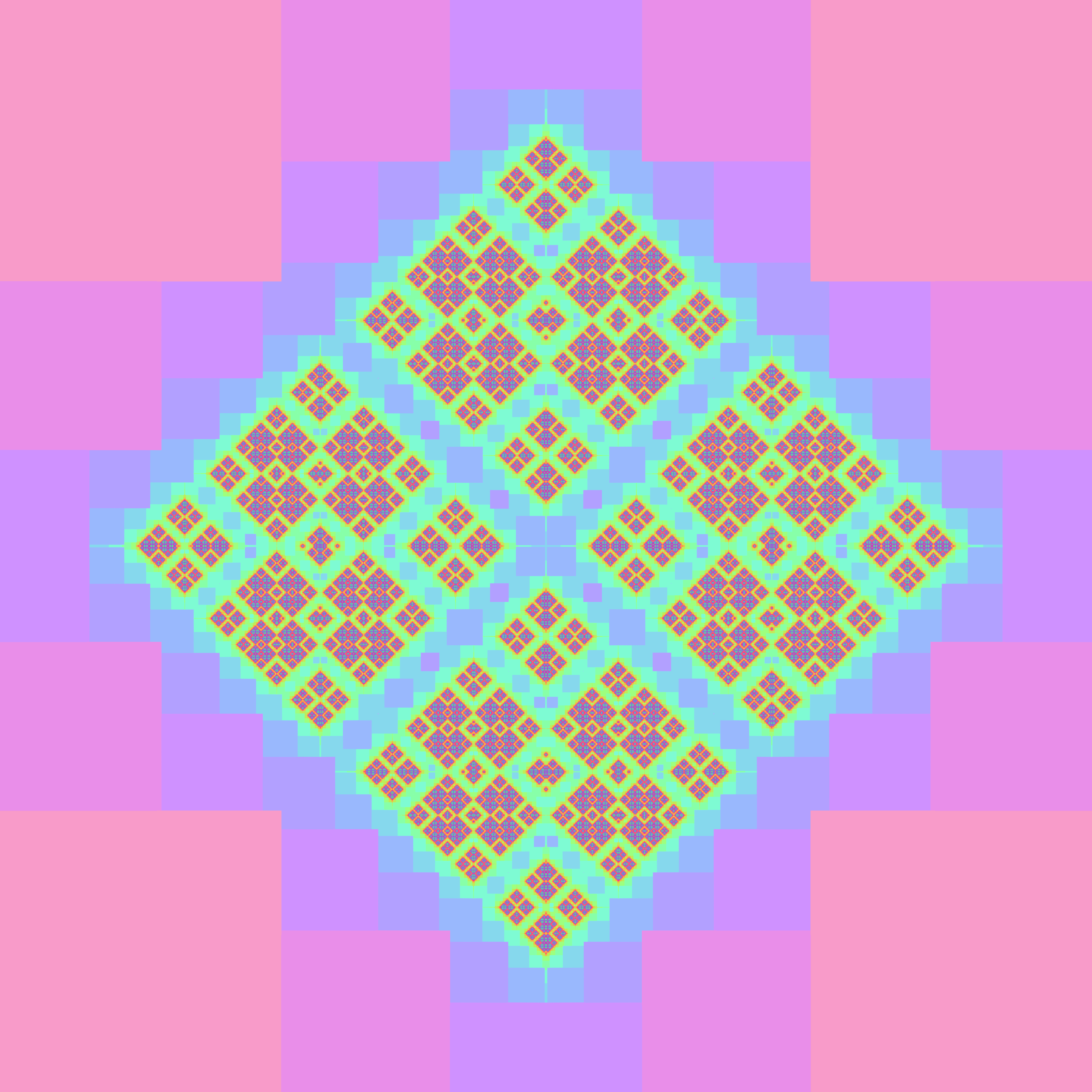
Here are some fun images we’ve made with it:


The animation features are mostly broken right now, but it’s more fun to find interesting states by hand anyway. Turn up the delay to get a mild turbulence effect of motion cascading down length scales, and put on some deep trance.
Here are some figures showing roughly what it does.


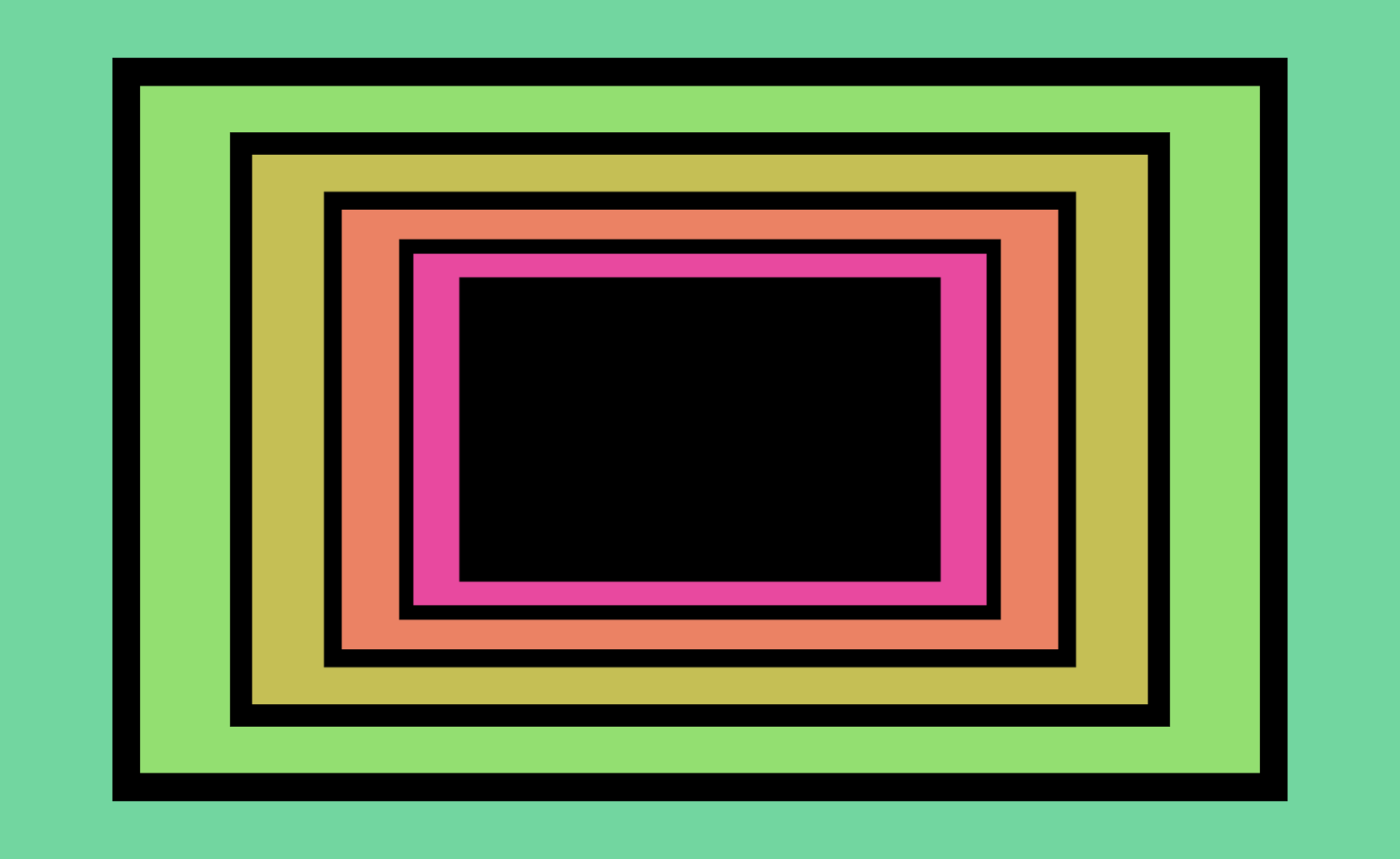
Figure 1. The first five iterations of the starting configuration. Note the shift in hue/saturation as the “iteration depth” increases.


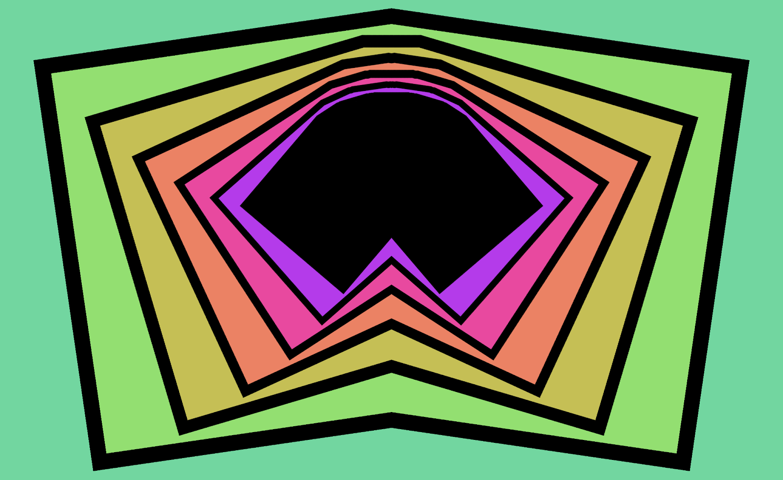
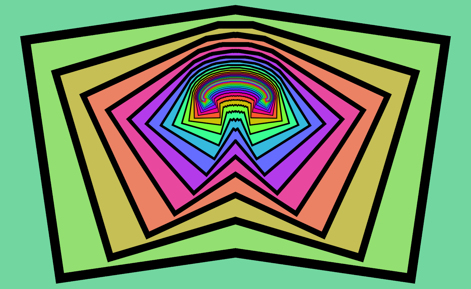
Figure 2. The first few iterations (and final result) of a configuration shifted slightly to the left and tilted, with the “X Mirror” effect on. Before each image is rendered, it is mirrored so that the right side matches the left side; otherwise, its rendering process is the same as that of Figure 1.
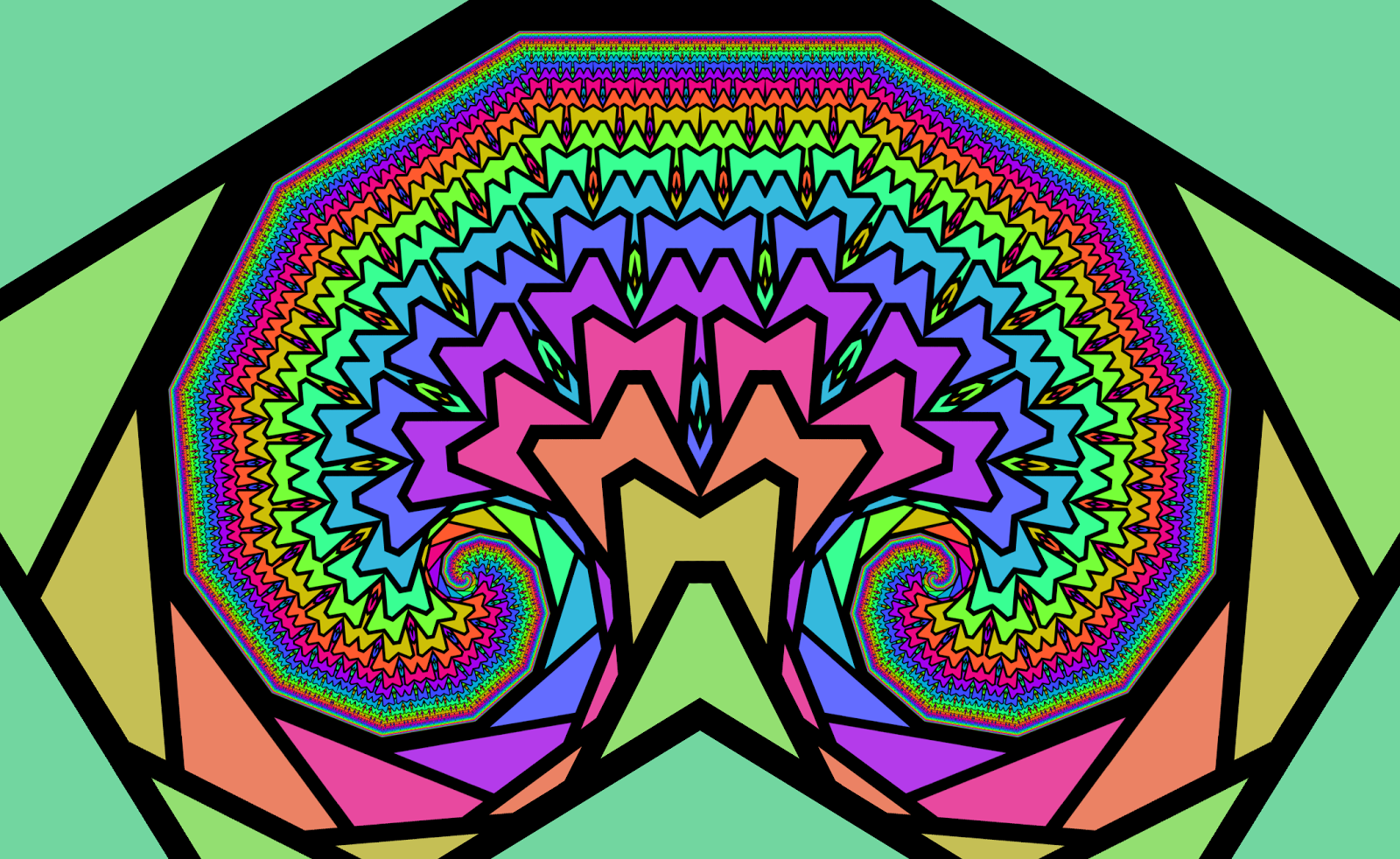
Figure 3. The “color cycle” transform makes the iteration depth apparent for different areas of the image.
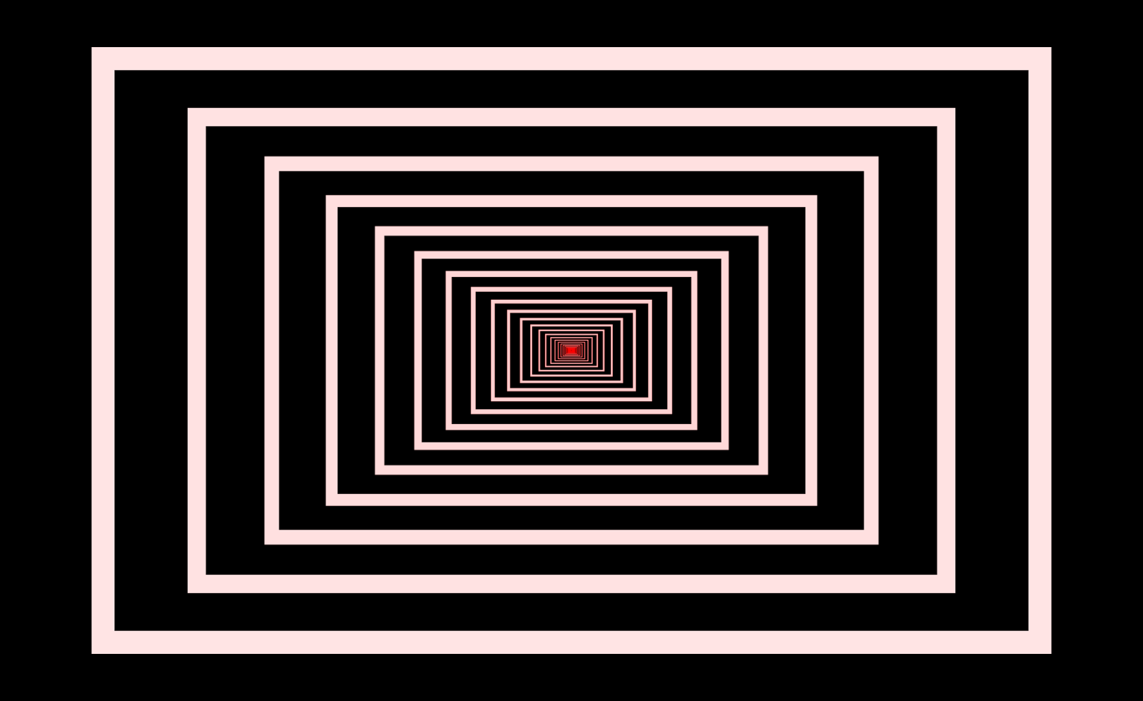
Figure 4. Here, the background color is set to black, and the border color is set to off-white with a slightly reddish tint. The “Color Cycle” effect is turned off, so the hue does not change with iteration depth. The gain effect highlights the fixed point of the configuration, which is a single point in the middle.
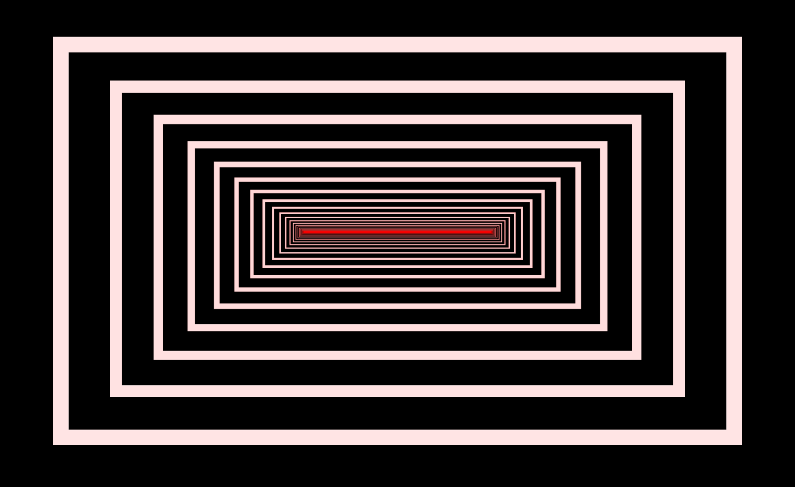
Figure 5. The same configuration as Figure 4, but with the center shifted to the left and the “X Mirror” effect turned on. The “fixed set” has expanded into a line segment.
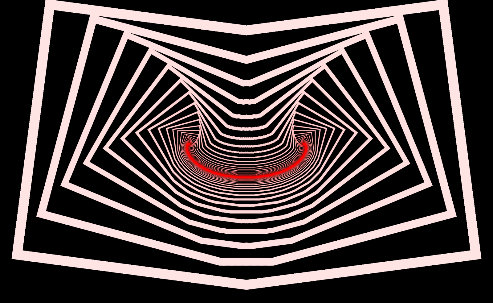
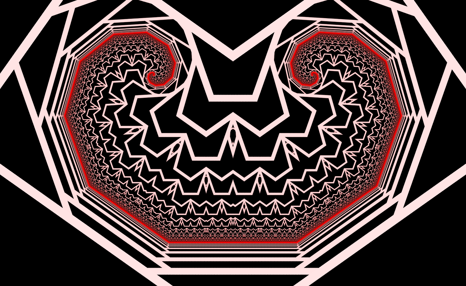
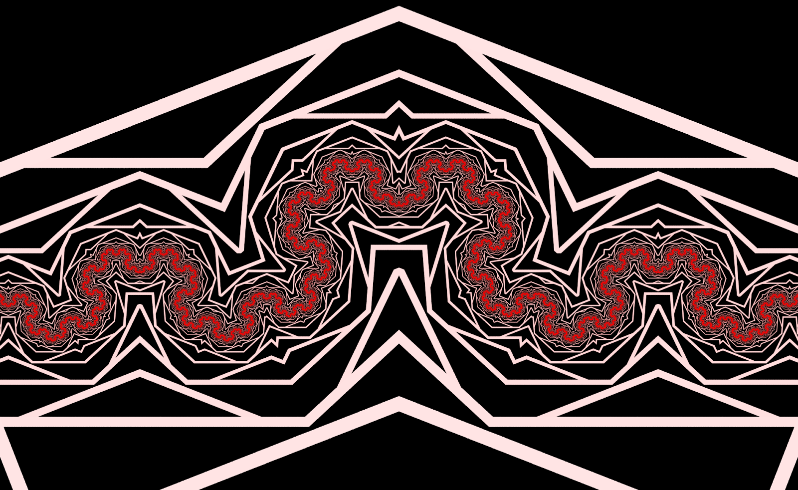
Figure 6. The same configuration as Figure 5, but rotated at different angles. The fixed set is evidenced by the bright red line, which takes on a fractal shape as its “total size” increases.
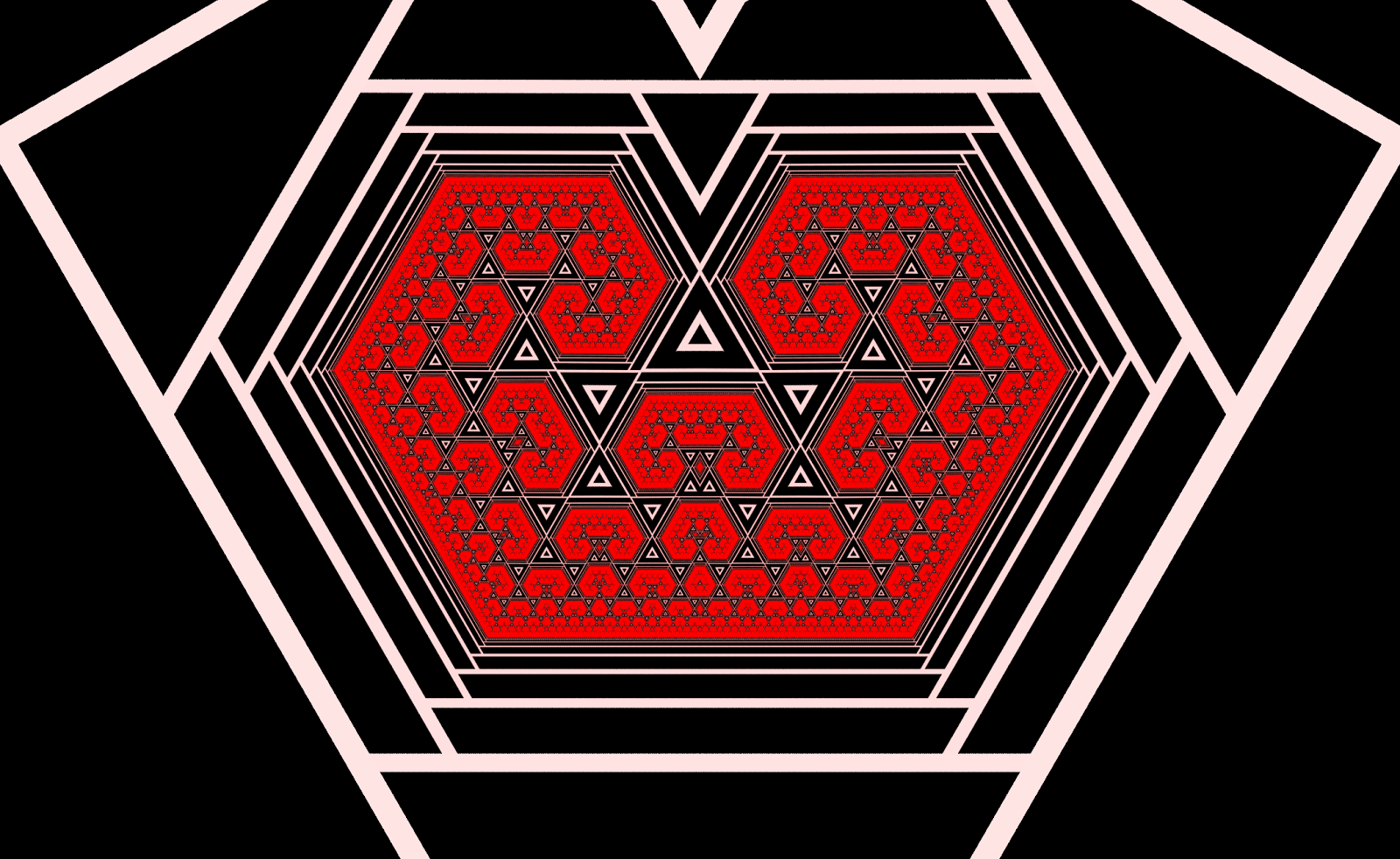
Figure 7. In some configurations, the fixed set takes up two-dimensional space at the resolution of the renderer.
An Experiment
Much of the intuition behind the video feedback simulator comes from simply playing with a real camera-monitor feedback system. It’s also a useful path to formalizing the system. So, here are some quick-and-dirty instructions for setting up an effective video feedback system using a camera and VLC:
- Plug in the camera and open VLC
- Start the camera video stream
- Go to File > Open Capture Device…
- Choose Capture Mode > DirectShow
- Select the webcam for Video device name
- Select None for Audio device name
- Adjust the video aspect ratio under Advanced options…
- Press Play and a window should appear with the stream
Start by tweaking the Essential > Image adjust settings so that colors don’t change when fed back through the system (e.g. nested images are the same color as the parent image). It may be easier to adjust your camera’s sensor settings directly.
Orient your camera to achieve a “picture-in-picture” effect. Try to keep the camera’s axis perpendicular to the plane of the monitor.
Adjust video color and effects under Tools > Effects and Filters > Video Effects or, if available, using utility programs provided with your camera.
For sharper edges, try increasing the contrast to make edges more pronounced.
To get the “gain” effect, try increasing the saturation slightly so that iterated colors are driven toward maximum saturation.
Try inverting colors on each iteration with Colors > Negate colors. This usually drives colors toward black and white, but other orbits are possible.
Try mirroring the image with Advanced > Mirror.
What’s happening?
The camera’s position, rotation, and magnification (scaling) factors define its view of the world. This view includes anything inside the camera’s viewing frustum, which is a rectangular pyramid that specifies what the camera can see. Whatever’s inside the frustum gets digitized by the camera’s sensor and transferred as an array of pixels to VLC.
VLC then modifies the pixels by applying local and global effects. Local effects are functions that transform a given pixel using only its previous value and those of other pixels in its neighborhood. Some examples are: color saturation, color negation, hue shift, and blurring. Global effects can source new pixel data from arbitrarily far away, and include mirroring.
Finally, VLC renders the pixels to screen. In order to produce feedback, these pixels obviously must be within the camera’s sight.
All of this processing and transfer can produce a time delay between between sensor record and image display, which affects how long the system takes to settle.
Phase Space
The dynamic (and sometimes chaotic) patterns produced from this experiment are generally controlled by:
-
The position, rotation, and size (scaling) of the “monitor rectangle” relative to the “camera rectangle”
-
Global pixel transforms (we’ll focus on mirroring)
-
Local pixel transforms (color shifts, inversion, &c.)
-
The record-to-render delay
For many configurations of these “kinds” of options, the rendered image eventually settles into some kind of pattern. But the overall structure of a pattern is overwhelmingly defined by the first two options, and not third or fourth: the local pixel transformations can dramatically affect the appearance of patterns – but not the underlying geometric structure. Changing the delay, meanwhile, only affects the time that it takes for the system to “settle”.
The first two options define what we call (in the program) a spacemap, or some sort of rule for taking one pixel and moving it somewhere else. The first option tells us that we need to take the “camera rectangle” and map it inside the “monitor rectangle” (or vice versa). The second option tells us that we need to take pixels from one part of the “camera rectangle” and map them over to another part of it by, say, flipping it across the a vertical line. A given spacemap represents a point in the phase space of this system, so we can classify our patterns by classifying parts of this phase space.
You will quickly notice that there are many configurations which either settle too quickly (when the “camera rectangle” doesn’t overlap enough with the “monitor rectangle”), or “explode” into large, intensely strobing regions. These are easily-classifiable sections of phase space, but they aren’t particularly interesting. However, you may sometimes notice fractal-like patterns “growing” out of an otherwise obnoxiously strobing region of space. What’s up with that?
Fixed Points
We are now in a position to more rigorously address what makes some of these images “interesting”.
For a given spacemap: if the “monitor inside the monitor” is smaller than the actual monitor rectangle, then we’ll call our spacemap “contractive”. On each iteration, all the features get a little bit smaller. For these states, we see either a finite number of iterations or an “infinite” number of iterations that tend to converge toward a subset of points. Without mirroring effects (or other global transformations), a contractive state converges toward a single point, or doesn’t appear to converge at all. The point of convergence is called a fixed point; it represents a point that the spacemap transforms back onto itself with every iteration.
But in our system we sometimes don’t see the fixed point because it’s “hidden beneath” another layer. More directly, we only see the fixed point if the monitor overlaps the position of the fixed point.
Obviously, it doesn’t actually matter whether we deal with a “camera rectangle” or “monitor rectangle”. Our monitor could have been circular, triangular, or whatever shape we wanted.
Global Transformations
What happens when we add mirroring back into the equation?
When you turn on a mirroring effect, the spacemap ceases to define a simple affine transformation: it’s no longer a nice, continuous, one-to-one map. So we can no longer count on there being only one fixed point.
The images below show an example of what happens when the Mirror X effect is turned on in our app:
Figure 8. A simple pattern without any mirroring effects. There is only one fixed point.
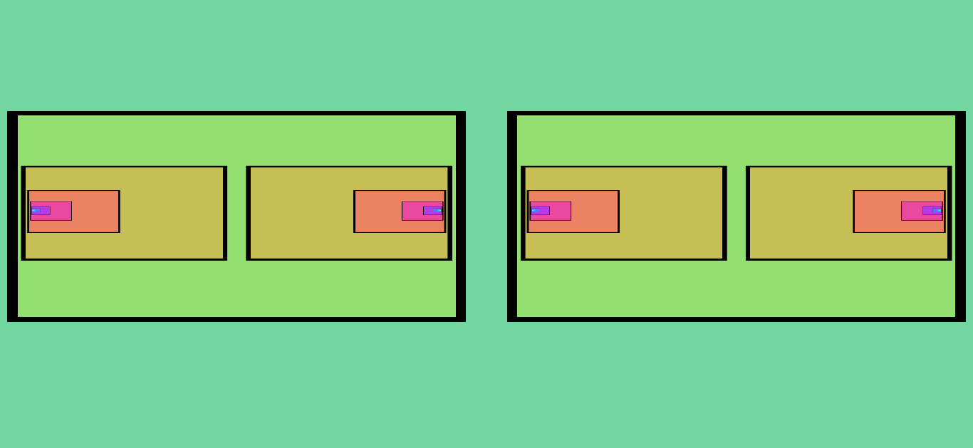

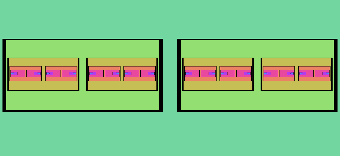

Figure 9. This shows the subsequent iterations (and final result) of Figure 8 after the “X Mirror” effect is turned on. The number of fixed points increases by a factor of two during each iteration.
Of course, we can also create a continuous set of fixed points, as seen in Figure 5. In many configurations, the fixed set itself forms the main “feature” of the resulting image.
The shape of a fixed set can be quite interesting; very often you will see fractal-like patterns emerge from the feedback app, as in Figure 6. Other software “fractal generators” are often visualizations of a fixed set itself (which is what Electric Sheep does, using iterated function systems).
But with the video feedback setup, we can also watch the convergence process toward the fixed set, and observe how the iteration layers interact with each other to produce the fixed set along with some neat patterns along the way. In some of the example images at the top of this post, the eye-catching features have more to do with the initial iteration steps than the shape of the eventual fixed set.
What we’ve found most interesting about video feedback is: the sheer complexity of the images it produces through such simply-defined and implemented spacemaps that really only have to do with the relative positioning of two rectangles. It’s somewhat intuitive, but always surprising.
This is all just scratching the surface of the mathematics behind the patterns that video feedback is capable of, but hopefully it’s good enough for a start!
P.S. You’ll notice that many of the “interesting” patterns contain regions of diverse sizes. That is, they appear to have a broad range of spatial frequencies. What’s up with that?
Space-time Dynamics in Video Feedback, James P. Crutchfield